How is Convolution?
Given two discrete lists of number or continuous functions, one can perform operations such as addition, multiplication, subtraction etc. But one of the most important operations we can do is the convolution of these signals. Why is convolution important and where does it show up in the physical world? From just signal and systems to image processing and even probability distributions, convolutions pop up very naturally. However, other very unexpected fields where convolution shows up is the solution of differential equations and polynomial multiplication.
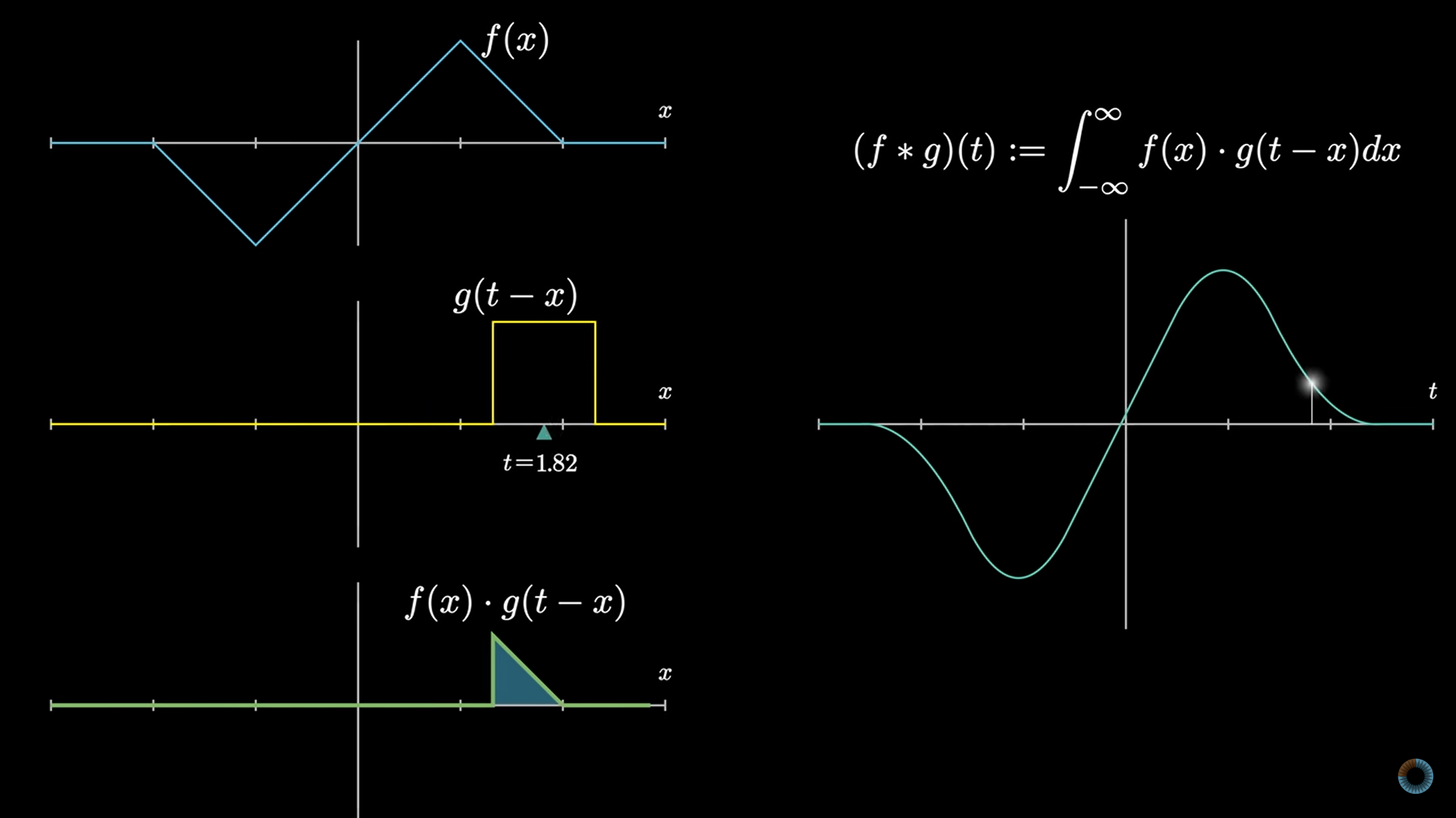
Convolution is something that is strived to be shown visually. Looking at the formula of convolution in case of continuous case,
\[(f * g)(t) := \int_{-\infty}^{\infty} f(x)g(t-x)dx\]Or in case of discrete case,
\[(f * g)[n] := \sum_{k=-\infty}^{\infty} f[k] \: g[n-k]\]Although scary looking, this formula just means to,
- Flip the second signal
- Shift it \(n\) times
- point-wise multiply the values
- add all of the values up

In the video given, Grant Sanderson talks only about discrete cases of convolution. In this case, the algorithm is very apparent to a “slide and sum” approach. Some examples of convolution can be seen hereafter.
Addition of Probability
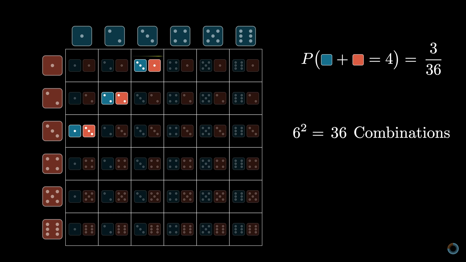
Dices are popular in the field of probability. We know that the probability distribution of a dice is a simple uniform distribution. However, if we have two die and we want to conclude the probability distribution of the addition of the two die number, it may prove tedious.

We can create a grid and then count the diagonals. But still the work is tedious.
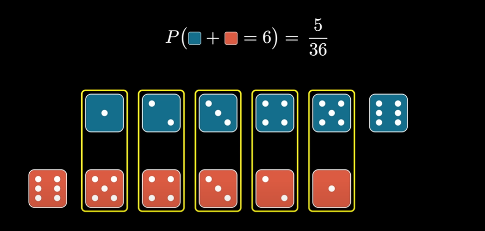
Another way of thinking for the same problem is by putting the dices row by row but flipping the second row. Then all the columns match up to be the exact same number. We can then easily find the combined probability. To find the the probability for some other sum we can shift the second row and find again the probability.

This process of shifting and multiplying and adding is nothing but the process of convolution. Thus, convolution is a natural way to express this kind of relation.
Moving Average & Image Processing
The idea of shifting, multiplying and adding is also a key in moving average. This is very trivial. We can also think of weighted moving average where the weight is much more in the center. This idea can be extended even further to image processing.
Considering an image which has to be blurred, we can simply define a 2D list or matrix of number. We can now shift, multiply and add to get the convolved value. This will in turn blur the image. If the matrix (also called kernel) is made in such a way that the maximum weight is in the center, like a gaussian curve, the blurring process is called “Gaussian Blur”.
Note: Convolution also requires one of the operand to be shifted. So technically, the matrix is shifted before the operation. However, most of these matrices are symmetric so this part of reversing can be skipped.
Not only blur, but processing any image for any features is done by convolving with some feature matrix. This is the basis for Convolutional Neural Network.
But why is this important?
Convolution is everywhere, but the process of convolution is still tedious. So, why the need of recognition of convolution operation is important. Simply because of one property of Convolution.
Considering $f(t)$ and $g(t)$ two signals,
\[\mathscr{F}\{ f * g\} = \mathscr{F}\{ f \} \times \mathscr{F}\{ g \}\]So, the Fourier Transform of two signals convolution is the same as first taking the Fourier Transform and multiplying it. This fundamental property of convolution allows us to do much more efficient calculation, where normal convolution of shifting and multiplying would take much more time then usual. One application of such idea is the multiplication of two polynomials.
Polynomials
Multiplying two polynomials is the same as convolving their coefficients. This can be trivially checked. Thus, a fast multiplying algorithm can be proposed to first do the Fourier Transform of the polynomial coefficients and then multiplying them, then getting the inverse Fourier Transform of the coefficients.
Consider two $n$th order polynomial. We can get $n$ different points from each of these polynomials. We can multiply them pointwise and get $n$ different points. Given $n$ points, it is trivial to find the polynomial. However, the complexity of the problems then shifts to solving a linear system of equation. This can be, however, avoided using the roots of unity and complex numbers. The approach is known as Fast Fourier Transform. This, however, was outside the scope of the video.
Conclusion
Convolutions are everywhere. From adding random variables to mixing signals for communication network. Using it’s property we can efficiently calculate most mathematical problems and we are doing so in everyday engineering.